Financial data isn’t scarce. Usable financial data is.
Financial services are among the most regulated industries in the world. Regulators instruct financial companies to make a vast amount of information public, enforcing strict requirements on what information needs to be shared. However, the instructions on how or in which structure this information should be shared are often vague.
The result? A plethora of valuable information lying in PDF documents, theoretically accessible to the public but practically useless for generating insights.
Traditionally, this gap has been filled by data brokers whose business model is to convert this unstructured, scattered data into a structured format available at a single source. For users, this has meant a stark choice: pay high subscription fees to data brokers or don’t use the information at all.
In this post, I’ll walk through how we built a workflow that converts PDF documents into structured, queryable data using Gemini.
The Challenge: Mutual Fund Factsheets
Mutual Fund monthly factsheets are a prime example. There is a tremendous amount of data made public by Asset Management Companies (AMCs) in these documents — Fund Managers, Benchmark Indices, Expense Ratios, and detailed Portfolio Holdings. Yet, extracting this data from 100+ page PDFs is a tedious, prone to errors and incredibly time-consuming.
We took up a project: KnowYourFund. Our goal is to mine this data into a structured format automatically, democratizing access to financial insights.
The Solution: Can we use NotebookLM?
Many of us have used tools like NotebookLM to query PDF documents and can imagine how perfect it would be for this task. We wanted to build something similar — an automated pipeline that could convert thousands of PDFs pages into structured data.
To achieve this, we leveraged the Gemini File Search API, which is essentially the closest API service to the power of NotebookLM.
Why Gemini File Search?
Implementing a Retrieval-Augmented Generation (RAG) system from scratch is complex. You have to handle parsing, chunking, vector storage, indexing, and retrieval.
Allowed us to:
Remove Complexity: The API takes away all the heavy lifting of managing vector databases and chunking strategies.
Accelerate Time to Market: We focused on the extraction logic, not the infrastructure
Lower Costs: By utilizing efficient filtering, we drastically reduced token usage compared to naive RAG approaches.
Live Demo & Future Plans
We have started by extracting information for a few AMCs and created a portal to showcase the extracted data.
We will be expanding this to cover more AMCs and showcase further insights, including features like “Ask Fund” (conversational queries) and cross-period analysis.
Replicability: Democratizing Document Search
The PDF data mining problem is not limited to Mutual Funds. Using this same structure, organizations can implement LLM search on their own documents as well. Consider it a custom “NotebookLM” for your company’s data.
This implementation of RAG by Gemini File Search API makes it accessible and affordable, leading to faster innovation across industries — whether it’s legal contracts, medical records, or scientific research.
If you’re working with document-heavy data — financial, legal, or otherwise — I’d love to hear how you’re approaching it.
For those of us who grew up in the 90s, Sachin Tendulkar wasn’t just a cricketer; he was a national event. Every time he walked out to bat, the world seemed to stop. His centuries weren’t just numbers on a scoreboard; they were markers of our own childhoods, moments of collective joy that taught an entire generation what it felt like to witness greatness.
Years later, I wanted to preserve those memories and create a tribute to this legend. To honor all 100 centuries, I turned to AI, exploring its API capabilities for large-scale content generation rather than using it as just helpful chat. The result is LittleMaster100.wordpress.com — a complete cricket blog celebrating each of Sachin’s 100 centuries with unique articles and custom AI-generated illustrations. This demonstrates how AI can transform raw cricket statistics into a complete multimedia storytelling website celebrating Sachin’s legendary career.
My Journey Through the Code
I built the entire website using a three-phase automation pipeline in Python. It was a fascinating challenge, and if you’re curious about the nuts and bolts, the complete source code is available on my [GitHub](https://github.com/hiteshgulati/LittleMaster100).
Here’s how I structured the process:
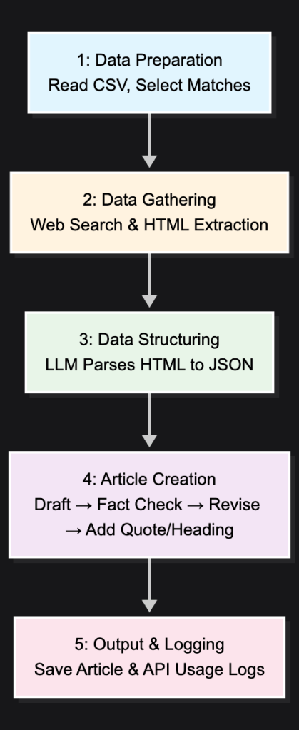
Phase 1: Writing the Stories — I fed the AI the basic match data from an Excel file. Its first job was to act like a sports journalist, searching the web for scorecards and old commentary. Then, it got creative, writing an emotional story for each match in the style of a famous author. To keep it honest, I even built in a fact-checking step.
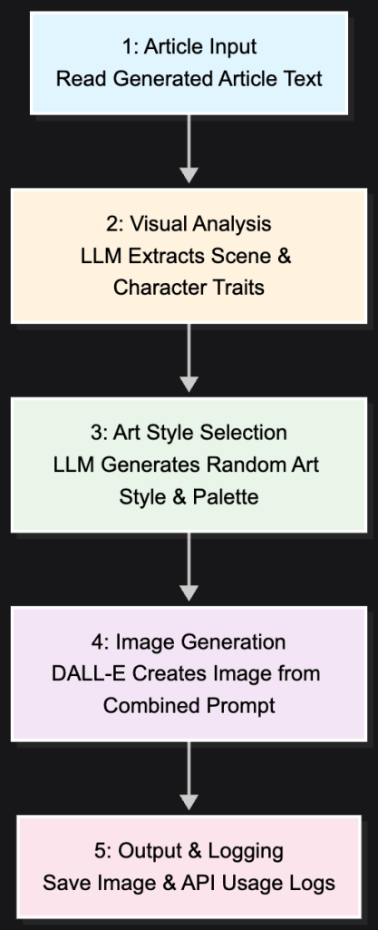
Phase 2: Creating the Art — For each article, I had the AI act as an art director. It would read the story it just wrote, extract the core emotion, and then generate a unique illustration using DALL-E. I programmed it to use different art styles and colors to give each memory its own visual identity.
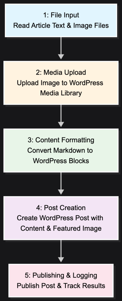
Phase 3: Publishing the Blog — Finally, a script takes the finished text and its corresponding image and automatically publishes them to the WordPress blog, complete with the proper formatting and a featured image.
The Economist
Cost of AI Content Creation
Phase
Time
Total Time (100 articles)
API Cost (per article)
Total Cost (100 articles)
APIs
Article Generation
~2 minutes
~3.5 hours
~$0.06
~$6.00
Tavily + OpenAI
Image Generation
~1 minute
~1.5 hours
~$0.04
~$4.00
OpenAI + DALL-E
WordPress Publishing
~30 seconds
~50 minutes
–
–
WordPress API
Total
~3.5 minutes
~5 hours, 50 minutes
~$0.10
~$10.00
Two things stand out:
Time: What would have taken months of manual work was finished in under six hours.
Cost: The entire project, a 100-article multimedia blog, cost just $10.
It’s a powerful illustration of how AI can bring large-scale creative projects within anyone’s reach.
My Takeaways
This project was a personal exploration of AI’s potential to be more than just a productivity tool. It can be a partner in creativity.
The results aren’t perfect. Some of the AI’s prose is a bit generic, and some of the images it created are, frankly, hilarious — more comic than inspiring. But that’s part of the journey. What started as a simple CSV file became a living website with 100 distinct memories, all brought to life with minimal human intervention.
For me, this proves something incredible: the entire content pipeline — from research and writing to visual design and publishing — can now be automated. It shows that we’re at a point where anyone can create comprehensive, professional-quality content. It’s a democratizing force for storytelling.
Ultimately, this was my way of saying thank you to a childhood hero. I hope you enjoy reliving the memories.
Attribution modeling helps businesses understand which marketing channels and customer touchpoints drive conversions. By accurately assigning credit to different interactions along the customer journey, companies can optimize marketing spend, improve ROI, and make data-driven decisions about their customer acquisition strategy.
Attribution Models
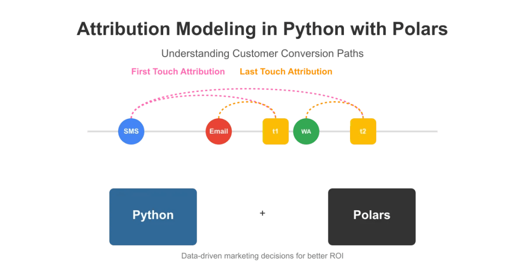
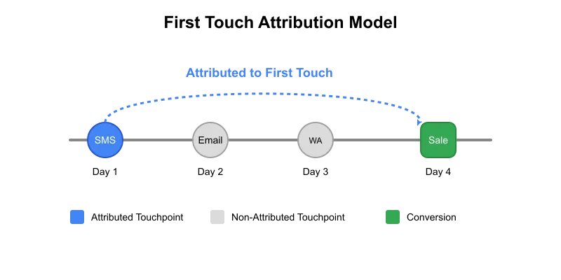
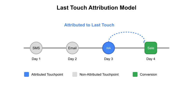
In this article, we’ll implement a simple yet powerful attribution model using Python and Polars. We’ll focus on two fundamental approaches: first-touch attribution, which assigns conversion credit to the initial customer interaction, and last-touch attribution, which credits the final touchpoint before conversion.
Conceptual Understanding
Let’s start with an example. An ecommerce company wants its users to complete transactions on its website. It runs campaigns targeting customers via SMS, WhatsApp, and email, requesting them to take action on the platform (in this case, making a transaction). All the requests or call-to-action communications sent to the customers are stored in a table. We name this table as call to action table or briefly CTA table. A sample version of the table would be:
| custID | channel | message      | timestamp  |
|--------|---------|--------------|------------|
| C1     | SMS     | Get 5% off   | 2025-04-01 |
| C1     | eMail   | Get 10% off  | 2025-04-05 |
| C1     | WhatsApp| Get 3% off   | 2025-04-07 |
Next, we have a table which stores all the actions or transactions performed by the customers. We’ll name this table as action table. Such a table would look like:
We sent three different calls to action (CTAs) to the customer, and in return, they performed two transactions. We want to see how effective these CTAs were. Based on the first touch attribution, both transactions can be attributed to SMS as that was the first communication sent to the customer. However, if we use the last touch method, transaction t1 will be attributed to email while transaction t2 will be attributed to WhatsApp.
The inner join operation in the first step creates duplicate action rows. We’ll need to remove the duplicate rows and keep only the attributed rows. The rows which will be kept depends on the type of attribution we need to apply.
First touch attribution: We’ll keep the earliest records based on cta_timestamp and then remove all other duplicate rows.
Last touch attribution: We’ll keep the latest records based on cta_timestamp and remove remaining.
# First Touch Attribution
result_df = (
    action_table_attributed
    .sort("cta_timestamp")
    .unique(subset=["txn_ID"], keep="first")
    .sort("txn_ID")  # Optional: sort the results by txn_ID
)
# Last Touch Attribution
result_df = (
    action_table_attributed
    .sort("cta_timestamp")
    .unique(subset=["txn_ID"], keep="last")
    .sort("txn_ID")  # Optional: sort the results by txn_ID
)
First Touch Attributed
custID
txn_ID
amount
action_timestamp
channel
message
cta_timestamp
str
str
i64
datetime[μs]
str
str
datetime[μs]
C1
t1
250
2025-04-06 00:00:00
SMS
Get 5% off
2025-04-01 00:00:00
C1
t2
175
2025-04-08 00:00:00
SMS
Get 5% off
2025-04-01 00:00:00
Last Touch Attributed
custID
txn_ID
amount
action_timestamp
channel
message
cta_timestamp
str
str
i64
datetime[μs]
str
str
datetime[μs]
C1
t1
250
2025-04-06 00:00:00
eMail
Get 10% off
2025-04-05 00:00:00
C1
t2
175
2025-04-08 00:00:00
WhatsApp
Get 3% off
2025-04-07 00:00:00
Step 3: Unattributed Actions
Not all actions performed by customers will be attributed to a CTA. Get all unattributed actions:
The final table contains all the actions done by the customers. Along with that, it also has CTA columns. Any transaction not attributed to any CTA will have null values in the CTA columns. This attributed table is helpful as it filters out which CTA communications are best for conversions and which are not.
Business Value of Attribution Modeling
Attribution modeling provides invaluable insights that directly impact business performance. By accurately identifying which marketing channels drive conversions, companies can allocate budgets more efficiently, focusing resources on high-performing touchpoints. This targeted approach typically increases conversion rates by 15–25% while reducing customer acquisition costs. Additionally, attribution reveals the customer journey, helping marketers understand how different channels interact and complement each other. This knowledge enables the creation of more effective, multi-channel campaigns that meet customers at critical decision points. Ultimately, data-driven attribution transforms marketing from an expense into a strategic investment with measurable returns.
Conclusion
In conclusion, implementing attribution models with Python and Polars empowers businesses to move beyond guesswork in marketing decisions. This approach scales seamlessly with growing data volumes while providing the flexibility to adapt attribution rules as business needs evolve. Remember that attribution is not a one-time exercise but an ongoing process that should be continuously refined. As your understanding of customer behavior deepens, you can progress to more sophisticated models like time-decay or position-based attribution. By turning raw interaction data into actionable insights, you’ll not only improve marketing efficiency but also enhance the overall customer experience — creating a sustainable competitive advantage in today’s data-driven marketplace.
Understanding the user journey is essential for any tech-enabled online platform.
We created an online platform where users can invest in mutual funds. On our platform, users can explore funds from various Asset Management Companies (AMCs) and choose the ones that suit them best. The process includes online KYC verification and finalizing transactions to invest in the selected funds. This journey is long and complex, leading to potential drop-offs at various stages. To improve the user experience, the analytics team must map this journey and identify friction points or bugs.
Here’s how we built our analytics pipeline to track the entire journey, identify drop-offs, and prepare daily business reports.
Events Table
The Events Table is the foundation for understanding the user journey. Every click, scroll, and action on the platform is logged, along with data from third-party webhooks. Here’s the table’s structure:
AnonymousID
CustomerID
EventName
EventMeta
Timestamp
AnonymousID is a temporary identifier assigned to users when they first visit the platform. If they log in, the CustomerID is also populated.
EventName indicates the specific action, such as a page visit, a button click, or a transaction confirmation.
EventMeta holds additional event data in JSON format, which can include various parameters like transaction amounts, page paths, or other details.
While the Events Table provides raw data, it’s challenging to extract insights directly from it. We created an enriched version with additional transformations to simplify analysis.
Creating a Flattened Table
To reduce complexity, we extracted key information from EventMeta into separate columns, creating a “wide but slim” table, also known as a Flattened Table. The flat structure allows analyst to write simple SQL queries using WHERE column_name = expected_value statement, instead of nested queries to extract JSON values
The flat structure allows analyst to write simple SQL queries using WHERE column_name = expected_value statement, instead of nested queries to extract JSON values
Here’s a Python snippet illustrating the flattening process with the Polars library:
variables_to_flatten = ['amount', 'AMC', 'transaction_charges']
dtype = pl.Struct([pl.Field(variable, pl.String) for variable in variables_to_flatten])

events_enriched = (
    events
    .with_columns(decoded=pl.col("EventMeta").str.json_decode(dtype))
    .unnest('decoded')
)
Stitching Missing Values
Due to technical issues, some rows in the Events Table may have missing data. Here’s an example:
AnonymousID
CustomerID
AA1
C1
AA1
C1
AA1
AA1
AA1
C1
In the above case, CustomerID is missing for some rows. Since AnonymousID AA1 corresponds to CustomerID C1, we can stitch the missing values by filling them from adjacent rows.
cols_to_stitch = ['CustomerID']
events_enriched = events_enriched.with_columns(pl.col(x).forward_fill().backward_fill().over('AnonymousID') for x in cols_to_stitch)
The result after stitching:
AnonymousID
CustomerID
AA1
C1
AA1
C1
AA1
C1
AA1
C1
AA1
C1
Persisting Values
In the journey, users make choices that can impact the subsequent steps. To capture these choices, we persist certain values for the remainder of the journey.
Here’s an example showing the impact of value persistence:
CustomerID
EventName
MutualFundSelected
C1
Landed
C1
MFSelected
Quant Active Fund
C1
InvestmentAmount
C1
KYCStarted
C1
TransactionCompleted
Even though MutualFundSelected is recorded only once, it persists throughout the journey until it changes. To persist such values, we use forward-filling:
pythonCopy code
cols_to_persist = ['MutualFundSelected']
events_enriched = events_enriched.with_columns(pl.col(x).forward_fill().over('AnonymousID') for x in cols_to_persist)
Result after persisting:
CustomerID
EventName
MutualFundSelected
C1
Landed
C1
MFSelected
Quant Active Fund
C1
InvestmentAmount
Quant Active Fund
C1
KYCStarted
Quant Active Fund
C1
TransactionCompleted
Quant Active Fund
Difference between Stitching and Persisting
Stitching and persisting are similar in that they both fill missing values, but they differ in their approach. Stitching includes both backward and forward filling, while persisting is only forward filling
Stitching: This technique is used when data might be missing due to technical glitches. It involves both forward-filling and backward-filling to ensure continuity of information, since the missing values can be confidently derived from adjacent rows.
Persisting: This technique is applied when certain values are expected to remain the same throughout the journey until they change. It uses only forward-filling because it’s uncertain what the value was before its first occurrence.
Stitching includes both backward and forward filling, while persisting is only forward filling
Extracting Key Events
To track business KPIs, we focus on three critical events:
Users landing on the invest section.
KYC initiation.
Transaction completion.
By creating separate columns for these events, we can easily monitor them:
The Events Enriched Table is the first step in building an analytics pipeline that helps map the user journey and identify drop-offs. This enriched table simplifies the analysis process by extracting and stitching critical information, persisting key values, and separating notable events for easy tracking. Although this table provides a wealth of data, advanced SQL skills and considerable compute power are required to extract insights.
In the next step of the analytics pipeline, I’ll discuss the Applications Table, where each row represents a single user application to invest in mutual funds, with all related information stored in a wider column format. This simplification allows for more streamlined analysis and easier business tracking.
Disclaimer: The above scenario is simplified and fictitious but closely resembles real-world scenarios often encountered when mapping customer journeys in online investment platforms.
In today’s globalized world, digital products have become an integral part of our lives. Whether it’s a sleek new smartphone, cutting-edge software, or access to your favourite content, the price we pay for these digital goods can vary significantly from one country to another. This phenomenon is often attributed to Purchasing Power Parity (PPP), and our analysis reveals some fascinating insights into how it impacts consumers around the world.
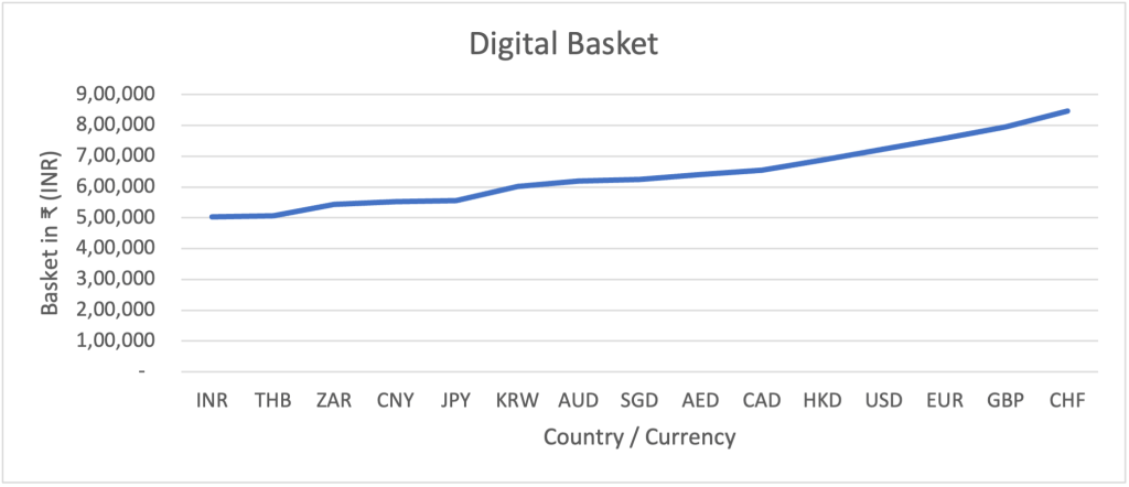
To understand the implications of PPP, we conducted an analysis of digital product prices in 15 different countries and created a basket of 13 products. This basket includes everything from smartphones to software and content subscriptions. In India, this basket would set you back ₹5 lakhs for a three-year period. However, the same basket in Switzerland would cost a staggering ₹8.5 lakhs (or CHF 9.2k) over the same time frame. The products in the most expensive economy are 70% higher than in the cheapest economy.
Factors Contributing to Price Disparity
Price disparity in the context of purchasing power parity can be attributed to two key factors: the cost of production and market pricing.
The cost of production encompasses all expenses incurred in manufacturing and selling a product, including manufacturing costs, logistics, selling expenses, and taxes.
On the other hand, market pricing is influenced by consumer behavior. In price-sensitive markets, consumers are less likely to purchase a product if its price is too high. Instead, they may opt for more affordable alternatives or even reconsider whether the product fits into their lifestyle. Conversely, in price-insensitive markets, consumers are willing to pay a premium if they perceive value in the product. For companies, the ultimate goal is to maximize profits, and they may adjust their pricing strategies to achieve this objective. They may set different prices for the same product in various markets. However, consumers are savvy and can take advantage of these price differentials. They may buy the product where it is cheaper and sell it in a more expensive market, effectively nullifying the company’s pricing advantage. Therefore, when setting prices, there’s always a trade-off between the effects of price sensitivity of the market and the potential for arbitrage opportunities.
To understand the impact these factors have on prices, we embarked on a journey to collect and compare prices of various digital products across multiple countries. This process necessitates the careful selection of products as we aim to create a diverse and equitable basket of goods that mirrors our digital landscape and provides valuable insights into the intriguing world of digital product pricing. In doing so, we can better understand how global economic factors and consumer behaviours shape the prices we pay for our favourite digital devices, software, and content.
Digital Basket
We focused on two key criteria when choosing products for our basket: representation and availability.
“Representation” means that the selected products should accurately represent the wide range of digital goods used in our daily lives. We want our basket to mirror the diversity of digital products we encounter.
“Availability” ensures that the products we’ve chosen are accessible to people all around the world and offer similar features and functionalities. This helps us maintain a fair comparison.
Following these principles, we’ve categorized the products into three main groups: Devices, Software, and Content. Each of these categories represents a distinct aspect of our digital experiences.
Devices
This category includes essential gadgets like mobile phones, laptops, and gaming consoles like the PlayStation and Xbox. These devices act as our gateways to the digital realm, allowing us to connect, work, and play. They are the tools that transport us into the vast world of technology.
Software
In our digital age, software plays a pivotal role in enhancing our productivity. Our chosen software products include Microsoft Office, Adobe Creative Suite, and iCloud. These applications empower us to create, communicate, and collaborate more efficiently. Whether it’s crafting documents, designing graphics, or managing emails, software forms the backbone of our digital workspaces.
Content
This category caters to our entertainment needs. It consists of platforms like Netflix, Amazon Prime, Spotify, YouTube, and Apple Music. These services provide us with a treasure trove of movies, music, videos, and more. What sets content apart from software is its primary purpose – consumption. While software helps us get things done, content is all about relaxation and enjoyment.
Head over to the Annexure to see the list of all products in our basket.
Studying the Pricing Disparity in Each Segment
Price Disparity – Devices
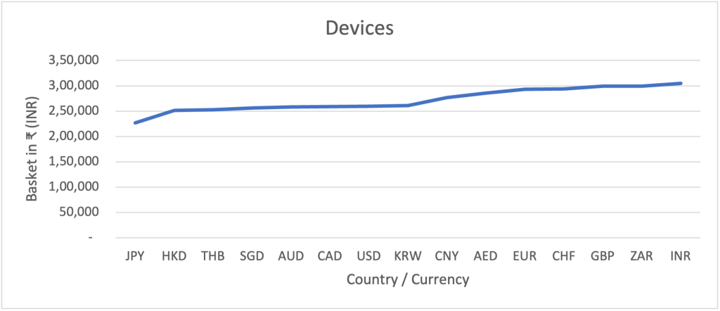
Our basket features must-have devices like the iPhone, MacBook, Play Station, and Xbox. Surprisingly, the cost of owning this tech treasure trove doesn’t vary much from one country to another. For instance, in Japan, the basket’s price tag hovers around ₹2.3 lakhs, while in India, it touches ₹3 lakhs. Although this may seem like a noticeable difference, the effect of price disparity in the device category remains relatively limited at a 34% increase from the cheapest to the most expensive country. Compare this to the disparity of 70% in the overall basket.
The production costs of devices are remarkably consistent globally, thanks to the efficient use of global supply chains by tech giants. However, market pricing reveals an interesting facet. While some markets may be more price-sensitive than others, these companies find it challenging to exercise significant price differentials due to a glaring arbitrage opportunity. The portability of these devices allows individuals to purchase them in countries like Japan, Hong Kong, or Thailand and resell them in India’s grey market at a lower price. In response, companies tend to maintain similar pricing levels across the globe to deter such activities.
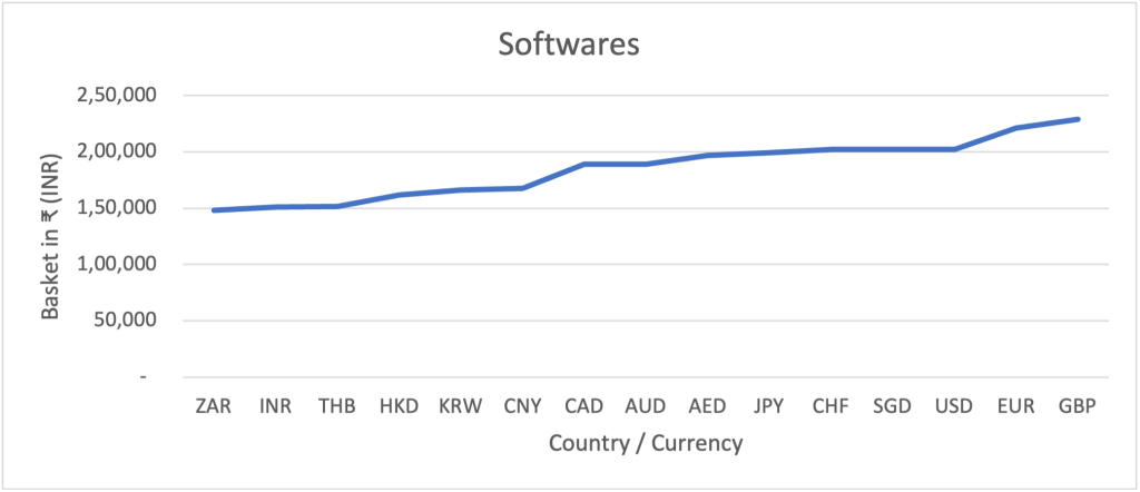
Price Disparity – Software
Our software segment encompasses three years’ worth of subscriptions to Adobe Creative Suite, Microsoft 365, and iCloud. Here, the price disparity is more pronounced, with South Africa offering the basket at ₹1.5 lakhs, while the same bundle costs ₹2.3 lakhs in the UK. The impact of this disparity stands at a noteworthy 55%.
Similar to devices, the cost of producing software remains consistent across the globe. These software packages are crafted at company headquarters and distributed digitally worldwide. Market pricing, however, presents a different scenario. The limited portability of software, enforced by digital distribution and IP address restrictions, enables companies to adapt pricing strategies that cater to varying consumer sensitivities. Consequently, these products are priced lower in emerging economies like South Africa, India, and Thailand, while prices soar in developed economies like the US, UK, and Europe.
Price Disparity – Content
Our final category delves into the world of content subscriptions, including Netflix, Disney+, YouTube, Spotify, and Apple Music. Remarkably, the cost of accessing these platforms differs significantly, with a 7x price differential between the most expensive market (Switzerland) and the cheapest (India). ₹50k in India compared to roughly ₹3.5 lakhs in Switzerland.
Content introduces unique dynamics into the pricing equation. Unlike devices or software, a substantial amount of content is produced locally, leading to varying production costs across countries. Additionally, like software, content’s distribution via the internet restricts portability, preventing customers from subscribing to services outside their regions. This distribution barrier empowers companies to further increase price disparities.
Conclusion
In closing, our journey through the world of digital products has unveiled a rich tapestry of price disparities, shaped by production costs and market pricing, reveal intriguing insights. While devices exhibit moderate variations in pricing across countries, software demonstrates more pronounced differences. Content, on the other hand, presents the most striking contrast, with prices ranging from a fraction of a lakh in India to several lakhs in Switzerland. This global interplay of factors highlights the intricate web that determines what we pay for our digital experiences. In this interconnected world, local contexts still profoundly impact our digital wallets.
Annexure
Devices
iPhone 15
Macbook Air – Apple M2 256GB Storage
Play Station 5 – Disk Version
XBOX Series X
Software
Adobe CC Subscription- Adobe CC All Apps Annual Plan Monthly Payment
Microsoft 365 Subscription – Microsoft 365 Personal Annual Plan
Apple iCloud Subscription – 50GB Storage Monthly Plan
Content
Netflix – Premium Plan per month
Amazon Prime – monthly Subscription
Disney + – Monthly Subscription
YouTube Premium – YouTube Premium with YT music
Spotify – Individual plan for 1 month
Apple Music – Individual for 1 month
The reason behind selecting these products for our basket is simple. They represent the core elements of our digital lifestyle, encompassing the tools we use to connect (Devices), work (Software) and the sources of entertainment that enrich our leisure time (Content). By monitoring the prices of these products across different countries, we gained valuable insights into how purchasing power varies globally, and how it impacts our ability to access and enjoy the digital world.
Business cycle is unpredictable, the return expectations, based on the previous 10 years, would probably be unrealistic in the future. Absolute return strategies, which are never supposed to post a negative return, posted –20 percent returns during 2008 financial crises. Investments that are supposed to be liquid actually—in extreme conditions like 2008— are not as liquid as expected and that their diversification strategies work only under normal market conditions. Such events call for a need of change in wealth management thinking and wealth managers need to change their definition of risk. Risk should not be defined mathematically as a standard deviation of return but as the probability of not achieving goals, which is the way that most people intuitively define risk. After all, although the volatility of returns is a matter of concern, it is not the same thing as failing to meet goals altogether. Thus, focusing on investors’ goals is a better way of wealth management. The industry was created by institutional investors who tended to have one goal: to meet their liability stream. All institutions—whether pension funds, foundations, endowments, or insurance companies—use their assets to defease a particular liability. Similarly for individuals should not think in terms of risk and return but in terms of dreams and nightmares.
Goals Based Investing is an investing technique which focuses on investing based on different goals of the investor.
Traditional Investing Approach
In the usual approach of investments, an individual invests in different funds based on professional advice and investor’s research. The allocation of these funds keeps changing as per investors age and market scenarios. Investors might also choose to consult a professional wealth manager for funds allocation. In both cases the objective of investments is to increase the capital to a target level while minimizing the risk. In such investments asset allocation changes to reduce the risk as the capital reaches target level or at the end of investment period for eg retirement of investor. This risk reduction leads to more investments in bonds/FD from equity. This ‘one-size-fits-all’ strategy is practiced by multiple wealth managers and AMCs across the globe. This easily followed strategy has number of flaws:
It does not take into factor the individual needs of investor. Not all investors might want to maximize capital, instead some have other objectives such as to repay their mortgage or buying bigger home or funding kid’s education.
It doesn’t account for capital appreciation before the investment horizon. For eg in case of unexpected bull run the capital will appreciate which might lead to high risk capability of investors.
It also doesn’t consider intermediate capital requirement of investor. Unexpected capital needs might present itself to investors such as in case of emergency, in such time the investments should be at certain level and sufficient liquidity.
Goals Based Investing – Introduction
Goals based investing recommends investors to set life goals and constructing a number of subportfolios for each one. That is, goal-based approaches are two-step approaches. First, the investor decides how to split his or her wealth among the different investment goals. Second, each investment goal is treated separately and a specific portfolio decision problem is solved. This considerably simplifies the portfolio decision process and investors are more likely to understand and follow their strategies. With goal based investing, the focus of the investment approach is on funding the personal financial goals. Goal based investing is similar to asset-liability management (ALM) for insurance companies and pension funds. The goals based investment redefines the risk for the investors. Risk should not be defined as the standard deviation of return but as the probability of not achieving goals, which is the way that most people intuitively define risk.
The goals based investing stands on two pillars:
Designing investors goals based on their needs and life style
Designing a methodology for goal oriented dynamic allocation strategy. This approach reduces the risks and improves the feasibility of the clients’ goals.
Designing the Goals
The first step in the process is to determine goals which will lead to optimal asset allocation. Simple goals might be like
Goal: I wish to save for retirement. The terminal capital at the retirement date is used to buy an annuity. This approach will follow traditional approach of capital maximization.
Goal: I wish to save for a mortgage. The capital will be used to pay off a mortgage at a fixed date. To minimize the downside risk of not being able to repay the mortgage, it is desirable to gradually transfer to a cash portfolio. The strategy in this case will be a stepwise reduction of risky asset classes to cash.
Goal: I wish to buy a house. Mix of risky and safe assets can be utilized for this goal. If the invested capital is not as per requirement at realization date, a smaller capital will also serve the purpose or alternatively the buying decision can be postponed to a relatively later date.
Goals can be more advanced in nature and can have multiple objects ranging from:
Critical component in the advanced goal based strategies is the prioritization of objectives or differentiation in the ability and willingness to take risk in reaching these goals depending on their importance:
Non discretionary goals: Non-discretionary goals need to be covered with a high level of certainty (80%-100%).
Discretionary goals: usually, small deviations from the target are not a cause for concern.
Exceptional cash flows may be conditional to the development of the capital. Disappointing returns lead to delay or redefinition of the objectives.
Investing for Goals
Once the investor has defined different goals, the investment strategy for each one of them can be different and dynamic. Goals demaning high level of certainity require safe investments, while goals which are flexible will have the appetite of relatively risker options. Flexibitliy of goals can majorly be attributed to timings and amount.
Goal A: These are the most sacred goals. Fixed nature of both Value and Timing signifies that the investor should have the exact defined amount at exact defined time, anything less or anything late wont suffice. Investments for such goals would include ultra safe options like digital gold. Planning for emergency situations like medical emergency also falls into this category and buying a insurance is also a great alternative.
Goal B: These are the goals which matures at a defined date but are flexible in nature of the value. An investor planing a vacation next year falls into this category. The maturity is defined which is next year but the value can be flexible which will ultimately define the destination. Such goals are best invested in relatively high risk investments but should be liquid enough to be realized well in time.
Goal C: An investor planning to buy a house will need to have a defined value but timining can be varied. Such goals are under this category and are best invested in relatively safer options but can be less liquid in nautre.
Goal D: Aspirational Goals comes under this category. Investor might want to achieve these but not able to suceed wont affect their lifestyle. The investment for these goals can be allocated to much more risker asstes.
While designing investment options for above type of goals following features of investments need to be factored:
Risk and return properties such as means, volatilities and correlations vary with the investment horizon. Based on data from 1802 to 1990 the correlation between nominal equity returns and inflation is negative for an investment horizon less than one year, negligible for an investment horizon of one year, and significantly positive for an investment horizon of five years. Also the volatility of equity returns decreases and the volatility of bond returns increases with the investment horizon.
Non-normal returns: mean-variance optimization assumes that returns are Normally distributed. However, empirical data clearly shows that return distributions have fatter tails than the Normal distribution, and are skewed.
Tail risk: correlations between asset classes increase in the left tails of the distribution. The 2008 financial crisis has shown us again that in bear markets the correlations between asset classes increase sharply. Consequently, the diversification effect which should protect a portfolio melts away in times of market losses, just when it would most urgently be needed.
Business cycle dynamics: For example, stock prices tend to lead in the business cycle while real estate returns typically lag in the business cycle.
Volatility of an asset class, like equity, is not a fixed characteristic. It is dependent on return levels. When equity return levels are negative, volatility is high.
Ignoring one or more of these real world features may impact the strategies adopted by the investors, resulting in incorrect conclusions and actions.
Conclusion
Use of Goals Based Investing approach is superior to the ‘one-size-fits-all’, target date oriented static allocation path used by most investors. The two pillars of the suggested approach: designing the goals: and designing investing strategy customized for each goal and dynamic in nature. This approach reduces the risks and improves the feasibility of the investors’ goals.
Debt based Mutual Fund schemes that invests in fixed income instruments, such as Corporate and Government Bonds are considered to give stable returns and are often proposed as an alternate to Fixed Deposits. In the last post here we saw these funds are also subject to market conditions and can depreciate in value during short periods. This price depreciation is caused by the prevailing interest rates in market, if interest rates increases bonds prices experiences a drop and thus the funds holding the bonds also drops in value. Similarly if interest rates decreases the debt funds will experience price appreciation.
As an investor just knowing when a price would increase or decrease is not sufficient, we would also like to know by how much. Let’s say we expect that after RBI’s next notification the interest rates would fall by 0.5%, we can deduce that the prices of debt based funds would increase so investing in these funds makes sense. But by how much the value would increase?, will the value of all funds increase by same percent or some bonds will have higher/lower impact? The answers to these questions lie in duration of the bond.
What is Duration?
Duration conceptually is the time the investor takes to recover their invested money in the bond through coupons and principal repayment. For example, consider a four-year bond with a maturity value of ₹ 1,000 and a coupon of ₹ 50 paid annually. The bond pays back principal amount on the final payment. Given this, the following cash flows are expected over the next four years:
Period 1: ₹ 50
Period 2: ₹ 50
Period 3: ₹ 50
Period 4: ₹ 50 + ₹ 1,000 = ₹ 1,050
If the market interest rates are at 7%, the fair value of this bond will be ₹ 932. The Macaulay Duration of this bond when calculated comes out to be 3.72 years. This means an investor who would invest ₹ 932 to buy the bonds will be able to recover their money in 3.72 years using the cashflows and principle payments.
Note: Macaulay Duration is often confused with the maturity period of the bond. For the above bond maturity period is 4 years which is the time when the investor will receive all the investment, Macaulay Duration is instead the period by when the investor will receive the amount they invested which is ₹ 932, the fair value investor paid to buy the bond. Macaulay Duration is thus always less than the maturity duration of the bond as invested amount will be recovered first and then the interest will be recovered.
What are the uses of duration?
The duration is an important concept in bonds market as it defines how sensitive a bond is to fluctuating interest rates. For example the above bond had following characteristics:
Maturity Amount: ₹ 1,000
Coupon: ₹ 50
Maturity Term: 4 years
Market Interest Rates: 7%
Fair Value: ₹ 932
Macaulay Duration: 3.72 years
Coming back to our original quest if an investor wants to know that what will be the fair value of the bond in case of market interest rate fluctuation. The answer is fair value will change approximately by change in interest rate * bond duration.
% Δ fair value = – (Δ Interest Rate * Bond Duration)
If the interest rates increases by 1% bond prices will approximately change by –(1%*3.72) = -3.72%. When calculated mathematically bond price moves to ₹ 901 (-3.5%). In other direction if the rates decreases by 1% bonds prices should change by +3.72% and when calculated mathematically if changes to ₹ 965 (+3.7%).
Conclusion
Duration of the bond can give investors a signal of what will be the impact of in market interest rates to prices of bonds and ultimately the debt mutual funds. The duration of debt mutual funds are generally reported in the fact sheets produced by AMCs which is helpful for investors to take investment decisions. An investor wants immunity from interest rate fluctuation would like to choose a fund with lower duration and investor who wants inflation protection in longer run would choose for fund with higher duration.
A debt fund is a Mutual Fund scheme that invests in fixed income instruments, such as Corporate and Government Bonds, corporate debt securities, and money market instruments etc. that offer capital appreciation. Debt funds are considered to give stable returns and have less risk compared to equity funds. These are often proposed as an alternate to Fixed Deposits and are advisable to highly risk averse people.
ICICI Prudential Bond Fund is a typical debt fund, its portfolio consists of government securities and top-rated corporate bonds. There is close to zero probability of default on these bonds and thus are quite stable while providing regular returns. At the start of this year (3rd Jan 2022) the Net Asset Value (NAV) of the fund was ₹ 31.87, and just one month later (3rd Feb 2022) the NAV stood at ₹ 31.38. How did the value fell by ₹ 0.50? We know that equity market is subject to market fluctuations and its value can go in either direction but how come value of debt fall? If we keep money in FD, its value is certain to rise then why not in case of debt fund?
To decode the situation let’s try to understand how a bond works. A typical bond is a contract between issuer and the current holder. The issuer seeks funds from the market and in return pledges to pay back certain fixed amount each year and a big final payment on maturity date. The issuer sets a par value of the bond say ₹ 1,000, issuer then pledges to pay a fixed rate say 5% each year, this fixed rate is formally termed as coupon rate. In case of ₹1,000, 5% becomes ₹ 50 which will be paid each year to the bond holder. Finally, issuer also agrees to pay the par value ₹1,00 in our case and at maturity say 10 years from now. The contract is then offered on sale in market and multiple buyers can place the bid to buy it. Let’s suppose a buyer buys this contract for ₹ 1,000 – the buyer will get ₹50 each year and ₹1,000 at end of 10 years, a rough calculation reveals that the buyer got 5% return on their investment by buying the bond. A return of 5% is better than what FD offers and thus a rational investor would prefer to buy the bond instead. Thus, more and more investors would rush to but the bond, but due to limited number of contracts only a few would be able to buy. Limited supply of this bond would create a situation where some investors might also be willing to pay more than ₹ 1,000 to get the bond. By paying more their return would be less than 5% but as long as it is more than FD rate a rational investor would still prefer this bond. If the FD rate is at say 4%, the stable price for the bond will be ₹1,081. On other hand if the FD rates were at 6% a rational investor would only pay maximum ₹ 926 for the contract and it will act as the fair price of the bond. Suppose an investor bought the bond contract at ₹ 1,081 when the prevailing FD rates were 4% but in short time banks started offering 4.5% on FD, the fair value of bond will now be ₹ 1,039, the investor will book a loss of ₹ 42. This is how value of a bond contract can fall and thus the NAV of a fund holding multiple bonds.
As in the example above the bond’s fair value is dependent on the prevailing interest rates in the market. If the interest rates increases in market investors would want better returns and thus would be willing to pay less for bond contracts marking a drop in bond’s fair price. While if the interest rate decreases the bond’s price would experience an upward movement. Thus bond mutual funds although being stable are impacted by change in interest rates.
How does a mutual fund works? An Asset Management Company (AMC) like Axis Mutual Funds pools money from various investors and manages that money by investing it into different options. All mutual fund have an investment objective for eg Axis Bluechip Fund’s objective is – To achieve long term capital appreciation by investing in a diversified portfolio predominantly consisting of equity and equity related securities of Large cap companies. Each fund is managed by a Fund Manager who decides when and where to invest the pooled amount while aligning to the fund’s objective. There is usually a team of skilled professional who assists the manager in taking investment decisions. AMC takes a cut from the pooled amount to cover its expenses this cut is usually around 0.5% to 2% of total asset under management (AUM).
To evaluate the investment decisions taken by the manager each fund has a benchmark index against which its performance will be compared. Axis Bluechip Fund which is supposed to invest majorly in large cap companies has its benckmark as BSE 100 and NIFTY 50. A manager is doing a good job if he/she is able to generate more returns than the index consistently by taking better investment decision.
Looking it from a different perspective: an investor have a choice to invest in mutual fund and pay for the expense ratio or directly replicate the index for free (or nominal cost) using their money. Rationally they would choose to mutual fund only if it has a proven track record of generating better returns. The difference between mutual fund’s return and index return is known as alpha. Simply put:
Alpha = Fund Return – Index Return
A positive alpha means rational investor should prefer fund and manager is proving his/her worth.
We compared returns of Axis Bluechip Fund to its two benchmarks over a period of 9 years. We defined different periods over while the return will be calculated and compared the number of days when fund had generated more return to days when index had more return. The observations are below:
Period
BSE 100
NIFTY 50
6 months
42%
44%
1 year
33%
30%
2 years
23%
17%
3 years
10%
6%
5 years
0%
0%
As per the above table: Historically BSE 100 generated better returns than Axis Bluechip Fund 43% of time (i.e. 43 out of 100 days). This number reduces as we take linger period and eventually drops to 0 if the period is 5 years. The the fund manager is generating better returns almost always in past if the investment period is long enough.