Goals Based Investing (GBI) is an alternate approach to investing and wealth management. As per GBI, the objective of financial investments should be to attain specific life goals rather than generating highest possible returns. These goals range from short term like buying a phone or a car to long term like saving for children’s education or building a retirement corpus. It highlights that the purpose of savings and investments is to fulfill future goals and all parameters of investment like risk appetite and asset allocation should be based on these goals.

Like in an IPL tournament the objective of any team is to land on top of the table, this objective is achieved by winning most matches and not just by hitting maximum runs. A team which won the most matches ranks higher on the table even if the other teams scored more runs overall or had better Net Run Rate. Teams having this clarity of goals are most aligned towards them and have better chances of winning the tournament. Goals Based Investing relates the same to individuals, i.e., having clear goals and aligning investments to fulfill them leads to a better life.

How to implement GBI in personal life?

List your Goals

It all starts with defining your goals, what you want in your life and when you want those things. Yes, it seems like a daunting task, but to make things easier we can start by looking at some obvious things, like we would retire by age of 60 and will need a retirement corpus by then, we would plan to fund children’s education when they turn 18, we would like to buy a big house when we turn 40 and so on. Once the longer-term goals are defined we can turn our attention to short term and lifestyle based goals like, we would like to buy a new car in three years’ time, we would like to go on a foreign trip after two years, we would like to re do furniture of our house next year, we would want to buy a new phone this year and the list continues. The beauty here is that we don’t need to list out all our plans at once, we can just start by listing a few and start planning towards them. In future as and when required we can amend or add new goals. To begin with,  we just need to get into the habit of describing the goal and planning towards it.

Plan to accomplish your goals

The goals we listed are like matches in an IPL season and we would want to accomplish all of them. But not all matches in a season are same. Some matches are more crucial than others, we definitely want to win the crucial ones while we can assume some risk in others. Some matches are against weaker teams, and we have some leverage to be more aggressive while others we need to be careful. Similarly, not all goals are same. Some goals are important for us like having a good retirement corpus or having funds for children’s education while others have less priority like buying a big house. In some goals we have leverage like going on a foreign trip, even if we are able to accumulate only 80% of the planned budget, we can always choose a more economical destination.

Once we have defined our goals, we can start to build a plan to accomplish them. Consider a crucial goal of buying a new car in three years’ time, we definitely want to buy a new car and will certainly need to have appropriate savings by then. It is similar to a team playing a crucial match and chasing a respectable total say 160 runs in twenty overs. The team here can’t afford to lose the match and thus would like to give charge to their most reliable batsmen. These batsmen might not be able to slog but has the best chances of chasing down the target. Similarly, to achieve the goal we would start saving a fixed amount each month and would invest that amount in a risk free / low risk instrument, an instrument which probably won’t give us best return in market but will generate appropriate savings in the given time frame most reliably.

Now consider another goal of say having a foreign trip in two years, again we definitely want to achieve it but we have variable target budget. This would be similar to a team batting first against a weaker team. They are confident that they can defend a target of 140 runs but still more the merrier. In this match they afford to take risk and send out sloggers in the initial overs. If they didn’t play well, we can replace them with defenders but on chance they slog good, we would stand to score more than 200. In investment parlance, we start saving a fixed amount monthly and would invest that in more risky but better returns instruments. In order to make sure that we achieve the goal we would keep monitoring our returns and if the instruments were not as per out expectations, we would switch to our beloved risk free / low risk instruments.

Consider another goal a non-crucial one, where we don’t mind even if we don’t achieve it. A team already qualified but playing remaining of the matches, winning is good for confidence but won’t affect its standing in points table. In such match the team would like to experiment with variety of different players. This might be helpful to test and spot good players. In investing we would like to try out more exotic instruments like small cap stocks or even future and options. It’s good if they generate good returns but even if it doesn’t we won’t be affected.

Thus, having our goals in place and categorizing them as crucial or non-crucial ones, or variable or fixed can help us to identify the risk appetite and the assets allocation (instrument selection). The benefits of GBI are generally realized when we consider many goals at once. Consider a scenario where we had two goals in parallel, buying a car and going on a foreign trip. The money saved for foreign trip is invested in instruments with better returns. In case we are lucky and get good returns, we might generate more than we require for the trip. We can then use the surplus money to buy even better car than we initially planned. Similar to the IPL season, it’s important to win matches, but while doing so if we can get more overall runs, then that’s a bonus.

 How to get started?

If GBI sounds interesting, and you want to start planning, then reach out to your investment advisor to develop an investment plan. We have developed an excel based model for you to play around some scenarios. This model is based on historical data and thus cannot be used to plan and monitor goals in real time. However, it serves as a good demo to play around with some scenarios and how things would have turned out in past if invested as per GBI. The link to excel model is here, it contains three screens:

Inputs Screen

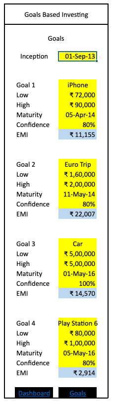
In the above screen, the user can input up to four goals that they want to plan and deploy.

• Inception date refers to date when the goals were entered, and user began saving for them on monthly basis.
• Low and high refers to the goal amount user wants to accumulate, to accomplish the goal user would want to have minimum of low amount and maximum of high amount, all funds generated above maximum will be transferred to other goals.
• Maturity Date is the date when the funds will be required for goals to be executed
• Confidence refers to how crucial the goal is, all crucial goals should have 100% confidence.
• EMI is the calculated part; it refers to amount the user will have to save monthly to accomplish the goal.

Dashboard Screen:

This screen gives an overview of all the goals.  The user has an option to choose current date and look how the investment would be doing at that day. The Market pulse tracks the market on selected date and Goals tracks the funds accumulated, total funds required and current status of each goal.

Goals Dashboard

The progress of each goal can be tracked here. The user can select any mentioned goal here and see in detail how that goal is progressing on any date. Value refers to how much funds have been accumulated till the selected date, and Days refers to how many days have passed since the inception date. Ideally, the value % should be greater than days % as we would like to stay ahead of the time.

Conclusion

The Goals Based Investing approach defines the role of investment as a tool to achieve future financial goals instead of just searching for best returns. Defining goals could start from jotting down the basic ones and adding more to the list as and when we identify new ones. Once the goals are defined and categorized, the planning can be initiated based on each goal. Crucial goals should use safer instruments while goals with some leverage could opt for bit riskier instruments. The performance of these instruments needs to be monitored periodically so that funds could be transferred to safer instruments in case required. Thus, the GBI approach helps to define the risk appetite based on the goals and enhances overall financial health of an individual.

Please use the linked excel workbook to play around with the concept using historical data and let me know your thoughts or suggestions.

Excel Model

It’s the first day of the month, and Shiva’s salary just got credited to his bank account. Earlier that amount would vanish by lunch on the same day because of Shiva’s huge credit card bills due to large EMI payments. Don’t get him wrong, he is not a shopaholic or someone who likes buying the highest priced item on the shelf. He is actually a smart consumer, buying only the product that he really needs after months of research.

A couple of years back, he needed a new phone. As usual, he started his research by going through the reviews of various models and visiting different vendors for the best deal. After diligent research of six months, he finally bought an iPhone on EMI. As expected, his Credit Card bill for the next month inflated and consumed a major chunk of his salary. That’s when he realized that he might be a rational consumer, but moneywise he is not smart.

While having dinner with his friends, Shiva discussed his EMI problem and how stressful it is for him to deal with it. That’s where he got introduced to a new concept of ‘Reverse EMI’. Instead of paying for the product after purchase via EMI, he can start investing a fixed amount of money into a mutual fund for the same period before the purchase, thereby creating a reverse EMI. By initiating the investment way ahead, Shiva thought that he could- (a) get sufficient time for product research; (b) postpone the payments during months with tight liquidity, and (c) generate good returns from the investment, effectively reducing the product cost.

It’s January 1^st, 2021 and Shiva is planning to buy a new phone later in the year. Based on his last purchase, he expects to spend around ₹ 1 lakh for this. He wants to buy the phone in October, and accordingly decides to invest ₹ 10 k every first day of the month. He invests this amount in a NIFTY based fund (a fund which tracks NIFTY 50 index) on 1^st Jan itself and is committed to do this every month.

It’s 1^st April, 2021, and Shiva has been diligently investing ₹ 10 k for the past three months. He is curious to know how his past investment is doing so far. Shiva feels delighted to know that his investment of ₹ 30 k (10k for 3 months) is now worth ₹ 31,234, giving him a profit of ₹ 1,234. Great, so he sticks to his plan till 1^st October sticks to his plan of adding instalment each month. When he withdraws his investment, he finds out that it’s worth ₹ 1,14,910. Wonderful, he uses ₹ 1 lakh to buy the new phone and keeps the ₹ 14k as bonus. The effective cost for Shiva: ₹ 86 k = ₹ 1 lakh he saved; minus ₹ 14 k he still has in his account. That’s equivalent of getting a discount of ₹ 14k.

Comparing the EMI and Reverse EMI process:

• In EMI, Shiva is obligated to pay the EMI no matter how his liquidity is. In reverse EMI, he can easily postpone his investment/purchase in case he is running short of surplus cash.
• The obligation created constant stress for Shiva, as missing a payment would incur high charges from the Credit Card company and would also impact his credit score. In reverse EMI, there is no obligation, and Shiva remains stress free.
• In EMI, Shiva paid ₹ 1 lakh for the phone, but in reverse EMI, he got an effective discount of ₹ 14 k. That’s unbelievable to his friends and Shiva gets appreciated for being a smart customer.

Shiva was a smart customer earlier; now he is also smart money planner.

Note: This is a fictional story to demonstrate benefits of implementing reverse EMI. The money movements however are based on actual market movements during the said dates.

In India we have more than 20 investment options available under different categories: wealth accumulation vs income generation, one time investment vs recurring payments, debt vs equity and so on. With so many options available at one’s disposal it can be quite daunting for someone to choose the best one for themselves. I’ll be adding a quick summary of all the investment options available and mention the pros and cons to help you choose the best one as per your specific needs.

I am referencing a book published by Value Research team by name of Best Investments

Banking

The investment options available by Banks are as follows:

Savings Account

A bank account is a financial account with a banking institution. The purpose of a bank accounts is to safeguard your cash and bring financial transactions to the banking network. With most of the transactions occurring within the network and government’s push towards digital’s transactions, bank account is assumed to be a must for all individuals.

Pro of having cash in the bank account is high liquidity – one can easily make quick transactions using the cash balance in bank account, there is no (or very little) wait time before transaction). Along with liquidity bank account offers safety and a moderate interest (around 3.5-4% pa) on the balance maintained in the account.

On other hand these interest rates are usually less than inflation rate (~6%) and thus account holders are losing money in real terms. Thus, in an ideals scenario you should determine your liquidity needs and only keep that amount in banks. The remaining balance should be moved to other higher interest rate options available.

Bank Fixed Deposit

A bank fixed deposit (FD) or term deposit, is an option in which bank keeps a certain sum of money with itself for a specified period of time. You are not allowed to withdraw or transfer that money during the time period. The main appeal for this option is banks offer slightly better interest rates (~ 4-5.5%) than savings account. This interest rates again are still less than inflation and thus investors end up losing money in real terms.

Bank Recurring Deposit

Bank recuring deposit is similar to FD the only difference being instead of investing a lum-sum amount, investors can choose to deposit a fixed amount every month on recurring basis. The interest rates offered by bank and lock-in period are in lines with same offered for FD.

Most banks these days offers a wide variety of other options as well which include Mutual Funds, Debt Instruments and Broker Account for Stocks. These although being offered by Banks are quite different from savings account or FD and thus, I’ll cover them separately.  

Post Office Schemes

Post Office Recurring Deposit

The Post Office Recurring Deposit (PORD) is a systematic savings plan, where you save small and equal sums of money each month for a period of 60 months. The savings attract fixed interest on capital (5.8% currently), which help investors generating assured sizeable savings over the fixed tenure of 5 years. The interest rates are usually close to inflation rate and thus investors don’t lose money in the longer run. The savings in PORD is guaranteed by the Government of India and thus can be assumed as risk free investment.

Post Office Term Deposit

The Post Office Time Deposit (POTD) is similar to a bank fixed deposit, you save money for a definite time period and earn a guaranteed return. The invested capital along with the compounded interest earned can be redeemed at the end of the tenure. The investment in POTD too is backed by government of India. Interest rates offered for the investment depends on the investment tenure (currently it ranges from, 5.5% for 1 year to 6.7% for 5 years). These rates are comparable to slightly better than the inflation and thus investors can expect to make a positive real return.

Post Office Monthly Income Scheme

The Post Office Monthly Income Scheme (POMIS) is a way to generate regular income from investment. You can deposit a fixed amount in POMIS and the interest earned is transferred back to depositor account every month. As there is a monthly cashflow generated in depositor’s account, this scheme is really good for someone looking to have a steady source of income. Currently, the interest earned on this scheme is 6.6% slightly better than inflation. A major limitation to the scheme is that maximum of ₹4.5 Lakhs can be deposited by an individual at a time, which amounts to maximum of ₹ 2,475 as monthly income.

Small Saving Schemes

Public Provident Fund

Public Provident Fund or more commonly known as PPF is a long-term savings instrument with a lock in of 15 years established by the central government with the objective to provide old- age income security. It offers assured returns (currently, 7.1%) and also has the exempt-exempt-exempt (EEE) status. The deposit made in the PPF account is exempted from income tax, interest earned on capital is exempted and finally the maturity amount if also exempted. This makes PPF a popular investment option, however there’s an upper limit of ₹ 1.5 lakh that can be invested per annum.  

Sukanya Samriddhi Yojna

The Sukanya Samriddhi Yojana (SSY) is specifically designed for girl child. The parents of girls aged 10 or below can open an SSY account in the name of the girl child and need to deposit minimum ₹ 250 to maximum ₹ 1.5 lakh per annum. The capital is guaranteed by government of India and earns an interest of 7.6% (currently). The SSY scheme also has the EEE status, i.e. deposits, interest earned and maturity amount all are tax exempted.

Senior Citizen Savings Scheme

The Senior Citizen Savings Scheme (SCSS), is a deposit scheme introduced by the Government of India to provide guaranteed and regular income stream for senior citizens post- retirement. The scheme is applicable only for senior citizens and then can deposit capital of up to ₹ 15 lakh. The capital when deposited is applicable for tax deduction, however the interest earned is taxable (over ₹ 50,000). The interest offered currently stands at 7.4%.

National Savings Certificate

The National Savings Certificate (NSC) is another scheme backed by the government. It is available with tenure of 5 years with interest rate of 6.8%. There is no upper limit for deposit, but it is tax deductible only up to ₹ 1.5 which is combined with PPF. It means if an individual is investing ₹ 1.5 lakh in PPF, they will get no deduction in NSC investment. This along with lower interest rates makes NSC an inferior scheme compared to PPF.

Kisan Vikas Patra

Kisan Vikas Patra (KVP) is a safe small savings instrument backed by Government of India. It has a tenure of 124 months which is 10 years and four months, which at current offered rate (6.8% annual) will double the invested amount. The money raised in this scheme is dedicated to be used in welfare schemes for farmers. There is no upper limit to amount invested however there is no tax benefit on deposit or on the interest amount. There is also a lock in period of 2.5 years after which amount can be scheme can be encashed by paying a penalty.

Pradhan Mantri Vaya Vandana Yojana

Pradhan Mantri Vaya Vandana Yojana (PMVVY) scheme (though marketed as a pension) is essentially a fixed deposit with LIC and has a guaranteed interest rate of 7.4 per cent for a period of 10 years. It is marketed as a pension scheme as interest rate generated is paid out in monthly/ quarterly/ semi annually or annually. There is no tax deduction on capital contributed towards this scheme and interest earned is also taxable.

Floating Rate Savings Bonds 2020 (Taxable)

The Floating Rate Savings Bonds 2020 (Taxable), popularly known as the RBI 7.15% Bonds, offer a 7.15 per cent taxable rate of interest over a tenure of seven years. They are called floating-rate bonds as the interest rate on these bonds is reset every six months. There is a lock-in for a tenure of seven years with interest payments done at half yearly intervals.

I am referencing a book published by Value Research team by name of Best Investments

Stress testing is a mechanism to test performance of a trading algorithm. During stress testing various unfavourable scenarios are designed and the trading algorithm is run over these scenarios and the Key Performance Indicators (KPIs) are measured.

The scenarios consist of internal events and external events, both have impact on algo’s KPIs. Internal events are events which occur within the system, it can include cases like delay in signal between trader and broker or even loss of connection between both parties. External events on other hand are cases which are not within the system like market related events, it includes cases like strong market movements or frequent price fluctuations.

Creating Scenarios

The stress testing scenarios are extreme cases which doesn’t occur in normal market conditions. Thus, in order to perform successful stress test, certain extreme market conditions need to be simulated. These simulations are created by varying values of different variables. The variables for internal events like delayed or loss of signal are built into the system and thus are incorporated directly during the testing process. Variables for external events like market movements and price fluctuations are needs to be designed externally and then are fed into the system during testing. We will describe the process of designing the data for these external events in detail.

Data Preparation for External Events

The variables external to the system are:

1. Market Movement
2. Market Volatility
3. Options Price Fluctuations

To design various scenarios values of these variables are used.

Market Movement

1. Upward movement – Market gains by 30% in one hour.
2. Downward movement – Market slips by 30% in one hour
3. Sideways movement (flat movement) – There is no net movement by the end of hour.

Market Volatility

Based on historical data Nifty has experienced intraday volatility of 19.6% (annualized). The variations in volatility variable are:

1. Low – Annualized volatility of 8%
2. Average – Annualized Volatility of 19.6%
3. High – Annualized Volatility of 50%

Options Price Fluctuations

Options prices are influenced by following parameters:

1. Price of underlying – Price of Nifty in case of Nifty Options. This is already considered this case in market movement.
2. Implied Volatility – Implied Volatility (IV) is perceived volatility of underlying by the market. This is generally close to actual volatility in the prices but may inflate or deflate in extreme market conditions.

Thus, to vary option prices variable IV is scaled as following:

1. Normal – No scaling to IV, i.e. IV is multiplied by 1.
2. Inflate – IV is inflated by a factor of 3. Thus, applicable IV would be Normal IV * 3.
3. Deflate – IV is reduced by factor of .33. Applicable IV = IV * .33

Using the variation in above variables, different scenarios are created. For each scenario price of Nifty and its options are calculated for each second for a period of one hour. This dataset can be fed into stress testing system to calculate algo’s KPIs.

The first season of Shark Tank India aired on SET India (Sony Entertainment Television). It featured seven investors or Sharks as described by the show who listen to entrepreneurs pitch ideas for a business or product they wish to develop. These self-made multi-millionaires judge the business concepts and products pitched and then decide whether to invest their own money to help market and mentor each contestant. The show featured total 121 ideas and of them 67 got funded. The total capital raised in the first season was ₹ 42.5 crores.

We analyzed how sharks invested their money in the ideas of their likings and created different categories based on their investment style. We present the Shark Tank Awards

Nominations – The Sharks

Ashneer Grover from Bharat Pe, Aman Gupta co-founder of boat, Anupam Mittal CEO of Shaadi.com, Ghazal Alagh co-founder of MamaEarth, Namita Thapar ED of Emcure Pharmaceuticals and Peyush Bansal CEO of Lenskart were the seven featured sharks for season one. The sharks invested their own money for the ideas they made the deal on.

Awards

The Big Ticket Shark

This shark paid the most amount for single idea. This shark was so obsessed with the idea that he didn’t mind what amount he ended up paying.

Note only the amount paid for equity will be considered.

Any Guess? Who wrote the biggest cheque?

DrumRollllllssss

Its Aman and Peyush for paying a sum of ₹ 1 cr. Aman paid this to buy his competitor Hammer Lifestyle while Peyush paid the same amount to Insurance Samadhan.

Big Shark of Small Pond

This shark bought the highest % of equity in the company, regardless of the money paid. This shark wants to be the big fish in a small pond.

And the big shark is:

Again Peyush Bansal. He invested ₹ 25 lakh plus ₹ 22 lakh debt for a whopping 75% stake in Sid07 Designs.

Small shark of Big Pond

This shark has the opposite approach of the previous one. This shark doesn’t want a huge stake, but is happy with a tiny bit stake in a big or potentially big company. This shark wants to be a small fish in a big pond.

The shark is:

Anupam and Aman. They both invested ₹ 50 lakh each to get a tiny holding of .75% for each of them.

Herd Shark

This shark prefers to collaborate with other sharks. This shark seeks approval and investment of other sharks before investing. This shark follows the hear. This shark made maximum investments when another shark was involved.

The Shark is:

Aman Gupta. He made total of 24 investments in which another shark was involved. But he is not far off, most sharks invested in collaboration with others. Like Anupam invested in 22 ideas along with other sharks.

Lone Shark

The brave shark, the shark who likes to go solo. This shark sees potential where other sharks doesn’t. This shark made maximum solo investments.

Any guess who the shark is.

Its Peyush Bansal. He made total 7 investments in ideas where no other shark was involved. Surprisingly the shark who came second is actually – the Herd Shark Aman Gupta who made 5 solo investments.

Greedy Shark

This is the real shark. This sharks want to get maximum equity % by paying the lowest rupees. This the shark among the sharks, the most greedy shark.

The award for being the most greedy shark goes to:

Vineeta Singh. She made total 16 investments and got total 136% equity across the companies by paying investment amount of ₹ 3.35 cr. She ended up paying average of ₹2.47 lakh per 1% of equity she received, the lowest amount per 1% of equity among other sharks.

Diversified Shark

Investments 101: Diversify your investment. This shark follows investment 101 to diversify their investment and buy in on as many ideas as possible. If one doesn’t work other might.

The shark who invested in most number of ideas is:

Aman Gupta, he invested in 29 ideas. He topped the table by a narrow margin of just one extra investment. Peyush who invested in 28 ideas came in second.

The Poor Shark

This is the poorest shark among all sharks. They invested least amount of money in overall season 1 of Shark Tank

The Poor Shark is, any guess?

Ghazal Goel, in total she invested ₹ 1.3 cr in the first season.

The Rich Shark

Saving the best for the last. This is the richest shark. This shark had deep pockets and splurged it all on shark tank.

The shark with maximum bank balance is?

.

.

.

.

.

.

.

.

Aman Gupta. He invested total ₹ 8.94 cr in 29 ideas.

Thanks for joining in for the Shark Awards this season. We’ll be back with more awards next season. Please suggest what other categories we should cover in next season.

If you think we should cover any other event for awards, please let us know in comments.

A trading algorithm has a defined set of instructions which needs to be executed in predetermined order. The profit generating capability might differ from one algorithm to another but widely all algos benefits from a faster execution. A python code can be developed to execute these set of instructions efficiently.

Let’s look on how to develop a python program to execute an algorithm. Generally, any trading algo will have three basic steps:

1. Fetch different variables like timing, price, quantity, volume.
2. Run a mathematical model like calculating candles, options greeks, etc.
3. Place appropriate trades if required (defined conditions are met)

We developed a module ‘Algo Module’ to execute all the above steps.

Algo Module

The Algo Module contains three functional classes, data_guy, events_and_actions and trader, one for each function.

Data_guy

Data_guy is a class whose objects will be responsible for fetching all required variables. It will periodically fetch, calculate and store variables which will be used by the algo.

Data_guy has following functionality:

set_parameters

A function to set various parameters of the class object.

update_data

This function fetches the latest data like last traded price, updated profit or loss, candle values etc. It also stores all the data which can be used for further calculation or logic.

get_atm_strike

This is a function to calculate strike of an option which is closest to the current traded price, this strike can be considered as at the money strike.

candle

This function calculates candles based on the candle length provided. It has flexibility to calculate candle of any length and for any historical time period.

calculate_greeks

This function is used to calculate options greeks. It can be used to calculate delta, gamma, rho, vega and theta of multiple options in single run.

Events_and_actions

Events_and_actions is the core strategy. The whole strategy is designed across multiple events and all events are mapped to an action. Events are designed to have multiple conditions, if all the conditions related to event are satisfied corresponding action is triggered. For e.g. if event_total_loss_reached is satisfied then action_close_the_day will be triggered.

If one event is satisfied during a iteration no other event will be checked, thus the events should be prioritized.

Events_and_actions have following functionality:

set_parameters

A function to set various parameters of the class object.

Events – event_1, event_2

These functions represents different events which needs to be monitored during the execution.

Actions – actions_1, actions_2

These functions perform different actions, like execute trade, square off existing trades. Action populate the orderbook with orders that needs to be carried out. It then call trader to execute those trades. Actions are mapped to different events and are executed only when its corresponding event is satisfied.

events_to_action

This function checks for all events one by one to see if its required conditions are met. If and event is satisfied the corresponding action is triggered.

Trader

Trader’s objects will be responsible to communicate with broker and carry out trades.

Trader have following functionality:

set_parameters

A function to set various parameters of the class object.

place_order_in_orderbook

This function iterates over all orders in the orderbook and places them to broker one by one.

strike_discovery

The function takes in price or delta as input and returns strike of option which is the closest match. It scans through multiple options and calculate their greeks and finally return the best matched strike.

get_positions

The function is used to get current position of the day.

Algo_manager

Algo_manager class is designed to initiate and set parameters all objects: data_guy, events_and_actions, trader. This class’ functionality is to manage above classes.

Algo_manager has just one functionality – to initiate and run the algo

action

Action function is meant to kick off every iteration for the algo. It triggers update data and then check for all events.

The Algo Trader is a WIP project, to access source code please check it out on github.

Algo trading is also known as  Algorithmic trading or automated trading, is a method of executing orders using a computer program that follows a defined set of instructions (an algorithm) to place a trade. The trade, in theory, can generate profits at a speed and frequency that is impossible for a human trader. The defined sets of instructions broadly includes three steps:

1. evaluates different variables like timing, price, quantity, volume
2. run a mathematical model
3. place appropriate trades if required (defined conditions are met)

A simple algo trader can have instructions like buy 50 shares of a stock if its price goes below 52 week average, or sell 50 share of holding stock if its price goes beyond 52 week high. A computer program can be designed to execute these steps and thus eliminate the need of human interaction. A typical infrastructure would consist three components.

1. A computer program which running on a laptop or deployed over cloud.
2. A broker terminal
3. Stock Exchange

The program connects to broker terminal which is further connected to stock exchange. The broker fetches market rates from the exchange and passes it on to the program. The program then runs computations on this data and send buy/sell trade signals to broker. These signals are relayed to the stock exchange by the broker.

As the code runs without human oversight there are multiple things which can go wrong during the market hours, for instance there can be large movement in the prices or there can be a connection error. To test the performance of algo under these extreme circumstances we perform stress testing. Stress testing is a computer simulation technique used to test the algorithm against drastic scenarios. Such testing is used to help gauge the risk and help evaluate safe guards and controls. It uses multiple scenarios which can be mix of historical, hypothetical, or simulated data. While testing, the algo is run over these scenarios to gauge its performance over some key performance metrices (KPIs). The scenarios thus should be designed to cover all internal and external factors which might have an impact on algorithm’s KPIs.

Designing Stress Test’s Scenarios

Let’s design stress testing scenarios for a sample trading algorithm. I covered an algorithm implementing Short Straddle Strategy here, it can serve as a good example. The short straddle algo buys and sells NIFTY options to generate profits.

Key Performance Index (KPIs)

KPIs for this algorithm will be how much profit or loss was incurred. We will be testing on unfavourable scenarios and so we would be more interested in knowing the losses and that too what would be the max loss incurred. Thus the first KPI can be Max Loss.

Loss distribution is also a key indicator of algo’s performance. While testing it on different scenarios we can measure what is the rupee loss incurred per unit of time, i.e. how much money was lost during 5 minutes of distress and if that is static, linear or exponential. Similarly we can also measure loss per unit of movement in NIFTY index.

The algo might have some safeguards built in which basically sense upcoming unfavourable event and suspends trading to avoid losses due to same. One of the key metric would be to check the reaction time of these safe guards, i.e. what level of losses are already incurred before these safe guards kicks in.

To summarize we defined three KPIs for the algo:

1. Max Loss
2. Loss per unit time and per unit of NIFTY movement
3. Reaction time of safeguards

Unfavourable Events

Unfavourable events can be internal or external to the system.

External Events:

External events are events which occur outside the system and have impact on algo’s KPIs. External events can include market movements and volatility, liquidity or price discrepancies.

Marker Movements can be categorized into three forms

1. Upward movement
2. Downward movement
3. Sideways movement (flat movement)

Market Volatility can be categorized into three forms as well:

1. Below Average
2. Average
3. Above Average

The market movements can be combined with each volatility to have 9 different scenarios, for instance one scenario can be Upward movement with below average volatility, Sideways movement with above average volatility and so on.

Options’ prices are heavily dependent on Implied Volatility, thus change in IV should be included as one of the external events.

Implied Volatility can be:

1. Below Average
2. Average
3. Above Average

Liquidity can have an impact on performance as it will limit algo’s ability to scale its current position or square off existing position.

Liquidity can be modelled as following:

1. Normal Liquidity
2. Dried Up Liquidity (Close to no liquidity)

There are times when market experiences absurd prices of an instrument, for instance an instrument which should have been priced are say ₹100 got sold for ₹2. In such cases if the algo hold such position a loss of 98% will be reflected and might lead to stop loss being triggered. The prices come back to normal very quickly but stop loss once triggered will stay active and might exit position at a loss. Thus occurrences of such freak prices should be included in external events.

Internal Events:

These events occur inside of the trading system but can have impact on KPIs. The system includes: computer program, broker terminal and the exchange. All three are connected via internet.

In such setup one of the internal event can be connection error between Algo and Broker or Broker and Exchange. The connection error can also be of two types, delayed signals or complete disconnection. Thus combining all we can have four types of events:

1. Delayed Signal between Algo and Broker
2. Delayed signals between Broker and Exchange
3. Connection Loss between Algo and Broker
4. Connection Loss Between Broker and Exchange

Another event can be high computation time for the algo, if algo takes a lot of time to run computation, any trade signals it generates will be delayed and might lead to unfavourable event. Factoring in such high computation time error into stress testing thus would be a good idea.

To summarize there can be five internal events:

1. Delayed Signal between Algo and Broker
2. Delayed signals between Broker and Exchange
3. Connection Loss between Algo and Broker
4. Connection Loss Between Broker and Exchange
5. High computation time by algo

Combining Internal and External events:

The internal and external events are independent in nature and so two or more of them occurring at same time is a possibility and would also be more adverse to the algo. For example there might be a case the market is having a downward movement and there is a connection loss between broker and exchange. Thus combining these independent events will lead to even more scenarios.

Conclusion

Algo trading can be implemented by reducing a trading plan into a set of instructions and converting it into a computer. The program can directly interact with broker for market data and trades thus eliminating need of human intervention. Lack of human control can lead to drastic losses in case of an unfavourable event and thus to test algo for such events we conduct stress testing.

Under stress testing we define KPI of the algo which might include Max Loss and Loss Distribution. The algo is run under a simulated environment where it is subject to different possible scenarios. These scenarios are can be external, internal or combination of both.

This post is an explainer on how to automate a simple task like sending a WhatsApp message to a contact and then scale it up i.e., sending similar message to multiple contacts.

We will be using Python script to automate the task and WhatsApp web as our delivery method.

Defining the task:

Send a new year’s greeting to 100s of contacts on WhatsApp, the greeting should contain an image with a meaningful message and personally addressed to the recipient.

Deconstructing the tasks into simpler defined and repeatable functions

1. Open WhatsApp web
2. Create Customized Image and save at a known location
3. Select Chat in WhatsApp web
4. Add image and send
5. Repeat steps 2, 3 and 4 for all contacts

Let’s work on each to-do:

Open WhatsApp web:

from selenium import webdriver

driver=webdriver.Chrome(chromedriver_path)

driver.get(‘https://web.whatsapp.com/’)

We have used selenium library to open the WhatsApp web, using selenium we can open browser instance interact with different elements and thus automate simple tasks.

Create Customised Image and save at a known location:

from PIL import Image

from PIL import ImageDraw

from PIL import ImageFont

def create_custom_image (source_image_path, text, font_path, size,

                            position, text_color) -> str:

    img = Image.open(source_image_path)

    edit_img = ImageDraw.Draw(img)

    my_font = ImageFont.truetype(font_path,size)

    edit_img.text(xy=(28,60),text,font=my_font, fill=text_color)

    edited_image_name = edited_image_path

    img.save(“edited_pics/” + edited_image_name)

    return current_path + edited_image_name

We are using Python Imaging Library for processing the image. We start by opening the source image using source image path provided into img object. Next we create another object as edit_img which is then used to add text, note that the text added is an input parameter and thus can be customized for each contact. After adding text we save the image to a known location and return the path back.

Select Chat in WhatsApp web:

def select_chat (name = “Hitesh Gulati”):

    search_box = driver.find_element_by_xpath(‘//*[@id=”side”]/div[1]/div/label/div/div[2]’)

    search_box.click()

    search_box.clear()

    search_box.send_keys(name)

    sleep(1)

    chat_table = driver.find_element_by_xpath(‘//*[@id=”pane-side”]/div[1]/div/div’)

    user=chat_table.find_element_by_xpath(‘.//span[@title=”{}”]’.format(name))

    user.click()

Coming back to WhatsApp, we search for the desired contact using the search box and click contact’s box to open contact window. We found the search box using its xpath which can be extracted by inspecting the element in Chrome browser. Once we searched for the contact, we can select the find box in the search results. Note that xpaths are dynamic in nature and might have to be searched again before using the code.

Add Image and Send

def send_image(file_path):

attachment_icon = driver.find_element_by_xpath(‘//*[@id=”main”]/footer/div[1]/div/span[2]/div/div[1]/div[2]’)

    attachment_icon.click()

    sleep(.5)

    image_icon =   driver.find_element_by_xpath(‘//input[@accept=”image/*,video/mp4,video/3gpp,video/quicktime”]’)

    image_icon.send_keys(file_path)

    sleep(1)

    send_button=driver.find_element_by_xpath(‘//span[@data-icon=”send”]’)

    send_button.click()

After selecting the contacts box, we can go ahead and send the customized image. We start by clicking the attachment button and then selecting Photos and videos from there. We will have to provide the saved image path to attach the image and then click the send button. All buttons attachment, photos and send button are referred using xpath and can be extracted using inspect in chrome.

Repeat steps for all contacts:

chat_list = pd.read_csv(“sample_list.csv”)

chat_list[‘sent’] = 0

for idx, each_chat in chat_list.iterrows():

    chat_title = each_chat[‘Title’]

    chat_name = each_chat[‘Name’]

    print(chat_title,chat_name)

    image_address = create_custom_image(text=chat_name)

    sleep(1)

    select_chat(chat_title)

    send_image(file_path=image_address)

    chat_list.iloc[idx,2] = 1

I saved all contacts in a pandas dataframe and created two columns. Title field is how I will search for the contact while Name field determines how the contact will be addressed. We loop through the list, create a customized image using Name field, select the chat using Title field and finally send the image. In the end we also tag the contacts for which the message was sent successfully, this will help us identify the contacts where the message was not sent.

We can use inspect feature within Chrome to get exact location of the search box and copy the full XPath related to it.

The Economic Limits of Bitcoin and the Blockchain

This article is based on the paper ‘The Economic Limits of Bitcoin and the Blockchain’ by Eric Budish. Please visit this link to access the paper.

Bitcoin Architecture

Bitcoin is an electronic cash system that’s fully peer to peer and works without a trusted third party acting as an intermediary. The basic workings of Bitcoin are similar to India’s UPI model: The sender initiates the transaction using their own public address (or UPI address), adds the recipient’s public address (or recipient’s UPI address) and finally approves the transaction using a private signature (in case of UPI, users use a PIN). This is a standard procedure and is implemented using modern cryptography.

While UPI uses a centralized authority i.e. the National Payments Corporation of India to authenticate and record these transactions, Bitcoin is a ‘decentralized’ network. The innovative idea behind Bitcoin was that its transactions are verified and publicly recorded without involvement of any trusted third party. Bitcoin uses multiple computers (or CPU) connected via network to verify transactions and create a public ledger by using blockchain technology. These CPUs are also referred as nodes. Every ten minutes, a large anonymous and decentralized collection of these nodes compete in a computational tournament for the right to add a new block of transactions to the public ledger. The problem is based on both the new block being added and the previous block added to the ledger. The first node to solve this difficult computational problem is declared as winner and reports both the new block of transactions and the solution to the computational problem. Other nodes accept this block and the whole tournament is restarted to add the next block in the chain. These nodes are owned by individuals or companies, they can also be referred as participants of the tournament. Each participant can hold any number of nodes all they need to do is add the buy the CPU and keep it running.

Each node in the tournament incurs a cost in form of electricity (consumed to keep the CPU running) for solving the computational problem. As an incentive to solve the computational problem, the winner gets rewarded in the form of newly minted bitcoins and transaction fees. Higher the number of nodes owned by a participant higher will be the cost and higher probability of winning. This activity of incurring cost in the hope to get rewarded is also known as mining and the participants as miners. Let’s convert this into a mathematical formula.

Presuming the following variables:

1. the reward per block = ‘P _block’
2. the cost of one unit of computational power = c
3. no. of nodes in the network = N

There can be any number of nodes in the system, but for the system to be in equilibrium total cost expensed should be roughly equal to total rewards. Thus, if N* is the optimal number of nodes, then:

Total Cost = Total Reward, or mathematically

N* c = P _block

The reward is distributed in the form of Bitcoin. So, higher the price of Bitcoin (in dollar terms), higher will be the reward for miners, leading to more energy consumption in longer run. It is also important to note that technological innovation that increases the efficiency of the Bitcoin mining process will not reduce the total energy consumption as a greater number of nodes are added. Also note that the number of participants can be less than the total nodes in the system as each participant can have more than one node.

Can the Bitcoin blockchain be attacked?

A dishonest participant can attack the system by creating an alternate chain faster than the honest chain. The alternate chain can reverse the earlier transactions and thus enable double spending (explained later). Now the probabilistically the likelihood of a participant creating an alternate chain and thus reversing z blocks exponentially decline by increasing z. Usually after couple of blocks it becomes improbable to attack the system and thus by waiting for an escrow period of two blocks is sufficient for payment confirmation. However, this is only true if majority of the blocks are honest i.e. the attacker controls less than 50% of the computational power.

What happens in case an attacker has a majority of the computational power? Even Satoshi Nakamoto’s paper states that an attack with more than 51% of computational power will succeed.

Cost of the attack

What is the cost of gaining majority computational power? If there are N* nodes in the system, the total computational power would be N* c. An outsider to gain a simple majority will have to bring in slightly more power into the system, thus total cost would be similar to N* c. While the attacker will be incurring this cost to attack the system in the process, they will also be gaining rewards of P _block per block and thus the net cost will be less than N* c, say α N* c where α is net cost per block. Now suppose the expected payoff to the majority attacker is V _attack, for the blockchain to remain safe the cost of attack should be more than the payoff:

α N* c > V _attack

The above equation captures that what enables the decentralized trust of the blockchain is the computing power devoted to maintaining it. The key thing to note here is that the security of blockchain is linear to the amount of expenditure on mining power. In contrast to other investments in security yield convex returns. Consider we want to keep products worth ₹ 1,000 safe, we can do that by using a lock wort ₹ 50, but if the products are expensive and worth ₹10,00,000 we will need a much better lock which will cost us more probably ₹ 500 or even ₹ 1,000. But essentially, we are able to have security of products worth 1000x more by investing 20x more on the lock (security system). This is called Convex returns and this is not tru foe Bitcoin which has a liner relation.

i.e. an analogous to how a lock on a door increases the security of a house by more than the cost of the lock.

Combining the first two equations:

P _block > V _attack / α

In other words, the equilibrium per-block payment to miners for running the blockchain must be large relative to the one-off benefits of attacking it. This puts a serious constraint on the technology. By analogy, imagine if users of the Visa network had to pay fees to Visa, that were large relative to the value of a successful one-off attack on the Visa network.

How an attack affects the system?

Before defining how the attack will affect the system, let’s see what an attacker can do and can’t do technologically.

As the attacker controls the majority of computational power, they can control what transaction gets added to the block and within computational limits remove recent transactions from the blockchain. The attacker even earns the block awards ‘P _block’ in the process. What the attacker cannot do is spend the bitcoin earned by other participants i.e. they cannot steal Bitcoins from other accounts.

Double Spending Attack

An attacker can manipulate the blockchain to their advantage. For example, an attacker gets into a contract to buy a new car by paying two Bitcoin. The attacker- (i) sends two Bitcoins to the merchant, (ii) allows that transaction to be added to blockchain, (iii) merchant delivers the car once the transaction is confirmed, (iv) the attacker can remove the transaction from public blockchain by building an alternate blockchain. The attacker can now spend the two Bitcoins recovered elsewhere, and thus the term double spending. Technically, the term ‘double spending’ is a misnomer because the attacker can spend the bitcoins multiple times.

The attacker in this scenario can maximize their gain by increasing the transaction amount and doing as many transactions as possible in a block. Assuming the maximum transaction size V_{transaction_max} and k transactions per block, maximum gain an attacker can realize can be k . V_{transaction_max}. The mining reward can also be divided across k transactions and assuming P _transaction is the reward per transaction the above equation can be rewritten as:

P _transaction > V _{transaction_max} / α

The value of α depends upon

1. Escrow period e, or the number of blocks attacker is trying to reverse, more the number of blocks more will be the cost.
2. Level of Super Majority A. The attacker can have simple majority or super majority. Higher level of majority requires more computational power and thus higher cost.

The author ran multiple simulations to calculate α, reported in Table 1. Panel C in the table represents net cost i.e. Cost of equipment – Block Reward. Let’s focus on e = 6 blocks or escrow period of one hour (6 X 10 minutes) and least majority of A=1.05. The net cost α = 2.33. Based on the equation above P _transaction > V _{transaction_max} / 2.33 ≈ 42% of V _{transaction_max}. This can be interpreted as implicit tax, if the maximum transaction size is one lakh rupees the transaction cost should be 40% or ₹ 40k. This is even larger percent on a cheaper transaction, if the transaction is small say ₹1,000, the tax is still applicable on the max transaction size and thus effective cost will be 400% in this case. Increasing the escrow period to say e = 1000 (around 1 week) helps to reduce this cost 1/53.5 ≈ 2% of max transaction, but it’s still substantial specially since all transaction will not be maxed out. To draw an analogy if same constraints were applicable on UPI payments and one needs to transfer ₹ 100, the transaction cost would be ₹ 200 (2% of maximum transaction of one lakh) and the payment confirmation would take one week instead of seconds as is the case with UPI.

Sabotage Attack

One rational given by the Bitcoin advocators is that a miner with more than 50% power is strongly invested in the system and thus has more incentive to keep the system running smoothly rather than attacking it. This does make sense. Imagine getting a news notification that says “Bitcoin network attacked: People lost Bitcoins received in last week”. Such news will sabotage the value of Bitcoin, resulting in a steep decline in its value. In the above scenario where attacker gained two Bitcoins from the attack, if the value of Bitcoin itself drops by say 20% (let’s call it Δ _sabotage) the attacker’s net gain will also reduce by 20% (or Δ _sabotage). The best-case scenario here will be that Δ _sabotage = 100% i.e., value of Bitcoin goes to zero and the attacker’s gain reduces to zero.

The attacker does stands to lose value due to sabotage, but there are many financial instruments available in market to hedge that loss and even the attacker can obtain speculative profits from holding a short position in Bitcoin futures. So, if one can attach a value to sabotage (V _sabotage) by speculative profits or other value gained externally, the attack will make economic sense. Bitcoin poses a threat to all the central banks across the world as they might lose their power of setting up the monetary policy, keeping this power would be highly valuable and thus high value of the collective V_sabotage.

Blockchain Mining Technology

In beginning, we assumed that the cost of waging the attack was similar to the cost incurred by miners to run the system or flow cost of the mining (α N* c). Here we assume that processing chips used for mining can be used elsewhere and hence once the attack is complete these chips will be deployed on other applications. However, in case of Bitcoin that is not true. At present, Bitcoin mining is done by highly specific and efficient chips called ASICs (application specific integrated circuits). These chips are more than 1000 times more efficient than general purpose chips and can’t be used anywhere else.

Since these chips are highly efficient, anyone planning to gain majority of the computational power will have to procure these specific chips. Also, these ASICs will be rendered useless after the attack and hence will have close to zero reusable value. The attacker will have to incur stock cost of these chips which is much higher than the flow cost assumed previously. The modified equation will now be:

N* C _{stock cost} > V _sabotage

The above equation states that security of Bitcoin relies on use of highly specialized equipment.

Collapse Scenarios

The increased security of Bitcoin due to increased cost can be nullified in three scenarios:

1. Ultra-cheap specialized ASICs

As the ASIC technology matures, Bitcoin ASICs might become very cheap and thus the cost would only be electricity required to run it which is equivalent to the flow cost

2. Efficient-enough general-purpose chips

As the popularity grows it is plausible that general purpose chips might become as efficient as ASIC. The gap might not close completely but even if it reduces to great extent, an attacker might invest in general purpose chips and put them to use elsewhere after the attack.

3. Value of sabotage becomes sufficiently tempting

As discussed earlier, many central governments might collude to sabotage the network as the collective value might become too high.

Conclusion

The anonymous, decentralized trust enabled by use of blockchain, while ingenious, is expensive.  In the double spending attack the implication is that the transaction costs of the blockchain must be large in relation to the largest-possible economic uses of the blockchain, which can be interpreted as a large implicit tax. The trust enabled by blockchain requires that the flow cost of running the blockchain is large relative to the one-shot value of attacking it. The attack itself might be more than the flow cost relies on Bitcoins use of scarce, non-repurposable technology which can make Bitcoin vulnerable to collapse if either condition change in the specialized chip market or if it becomes economically important enough to tempt a saboteur.

Overall, the results place potentially serious economic constraints on the use of the Nakamoto’s blockchain innovation. Most businesses and governments presumably have access to cheaper forms of data security, e.g., distributed ledgers or databases that require a trusted party (e.g., the business or businesses themselves), rather than having to pay the high costs of the trust that is emergent from a large network of untrusted computers coordinating on maximum proof-of-work.

₹ 71,962. This is the amount Short Straddle Strategy could make in three months if one is willing to engage a capital of ₹ 7,00,000. Seventy thousand rupees in three months on seven lakhs makes a monthly return of 3.4% and an annual return of 40%. I know, you would say “40% return? that sounds crazy!” To that, I would add: It’s not crazy, it’s ridiculous.

We are able to generate these returns by selling options as per the short straddle strategy. The whole process is really easy once we understand the basics. So, let’s begin with absolute basics

What are options?

Options are financial products and like company’s share, it can be bought or sold on exchanges including National Stock Exchange (NSE).

Generally, when two parties buy and sell company’s share, both have opposing views. The buyer believes that company’s shares are trading at a lower price and that price would increase in future. Thus, it’s in buyer’s interest to buy the share now at prevailing lower prices. The seller on other side views company’s shares to be trading at a higher price and expects that to go down. Thus, the best time to exit is not at current high price. As time passes and the share price moves, either the buyer or the seller stands corrected and thus makes profit on the deal. Consider a transaction where Sameer the seller sold shares of Reliance to Bobby (the buyer) at ₹ 2,500, next if the price moves up by ₹ 500, Bobby’s view stands corrected, and he will make a profit of ₹ 500 as he can now sell the same share at a higher price.

Options are different as it brings the element of time into the transaction. Like shares, the two parties buying and selling options in the market have opposing views, but the views are a bit different in this case. The buyer of options believes that stock price will move and defines a time period by when that move is expected. So, for buyer to win these two conditions need to be true a) stock price will move (move up or down) and b) within a defined period of time. The seller on other side of the table will win if any of these two conditions are not met. Consider a transaction where Bobby the buyer buys option from Sameer the seller saying a) Stock price will move up by 500 points or more and b) This will happen in next three days. On the third day if the price is up by 500 or more Bobby wins and thus stands to make profits, else Sameer will book profits. Note that if price doesn’t move by third day but did on forth, still Sameer wins as the second condition was not met.

What is Short Straddle Strategy?

Options unlike shares can have different properties. Options can be either call or put, each option has an expiry date and a strike price. These properties make options highly flexible. We can group multiple options having different properties to form a strategy representing our view of the stock prices, we call this group an option strategy. Short Straddle is one of the strategies.

When using the Short Straddle, our view is that prices will remain stable for good amount of time. Once we enter the strategy the longer price remains stable higher are the profits, on other hand if it (stock price) become volatile soon after entering, we can expect to lose money as well.

During a trading day the stock price movements drifts between being volatile and stable multiple times. Our target using the short straddle is to deploy the strategy during stable period and stay away during a volatile one. Thus, price movements are the key to make profits. So, do we know how to predict the price movements? Quite frankly NO. But on the brighter side we know a way to get around that.

What’s our secret sauce?

What to do when we can’t predict movements? It’s simple learn from history, take calculates risk and lastly be quick if we are mistaken. Here’s how we implement this plan:

Historically the stock prices are volatile during initial minutes of the day, thus we avoid entering the market at start. After the initial agitation probability of prices being stable increases, thus, we are ready to deploy and wait for prices to reach an optimal range. Once it hits that range, we send out buy/sell market orders for options to deploy the short straddle strategy, at this point we say that we have taken a position. While our strategy is deployed, we want the stability in movements, if stable we earn money but if prices are volatile, we can also incur losses. Since there is no certainty, we keep tracking the price movements. If it is stable, we would sit tight and keep booking prices, but the moment we feel that prices are becoming volatile and moving beyond our comfort zone but need to either switch our position to have a new comfort zone or exit the market entirely. By switching our position, we incur small lose but continue to stay active thus keeping the possibility of getting profits alive. If we choose to exit the market, it’s like turning off our devices and calling it a day. We like to equip with both the options and take appropriate action based on the prevailing conditions.

As an additional layer of safety, we also define a loss limit. There might come a day, a bad day, when most of our calls are mistakes and we keep losing money on each position. We want to end a day like this as early as possible. The loss limit comes into play here. Suppose we define a loss limit of ₹ 2,000, any given day the moment we incur a loss of this limit we will make an exit.

The key here is taking swift action, by quickly switching our position we ensure we have the most optimal strategy in place. The quick exit order on hitting the loss limit puts a cap on total loss for the day and thus we have the confidence that one bad day won’t ruin our overall profits. This here is our secret sauce, being quick to flex our strategy as per the prevailing conditions.

If we are relying on being quick, we know that we need to be really really good at it, and this is the reason we follow three steps repeatedly a) Track the market, b) Analyze the conditions, and c) Take appropriate decision. These steps although simple takes time for a human to process and implement and thus there are two additional elements to our plan:

Algo Trading

An algorithm is a set of logical instructions entered in a machine for it to follow. In algo trading, we code the three steps it into the computer and run it repeatedly. Computers although dump in intelligence are very fast when it comes to processing. By letting machines help us we are able to run all three steps track, analyze and act in less than a second and thus performing the whole task sixty times in a second or three thousand six hundred times in an hour. Say we entered a position at 9:30:00 AM, we will track, analyze, and act at 9:30:01 AM, again at 9:30:02 AM and again at 9:30:02 AM and so on.

Liquidity

Running an algorithm ensures that we are taking correct actions and doing it in timely fashion. Suppose there comes a situation when algo decides to take an action, maybe to switch a position or exiting the market, the algo by itself can only place market orders, we still need to rely on market for orders to be fulfilled. These actions will be frequent and thus market needs be ‘Liquid’. Liquidity of market is a feature whereby one can quickly purchase or sell products at fair price. In a highly liquid market one can expect all the orders to be fulfilled almost instantly which is the kind of support we need from market.

To ensure we have sufficient liquidity while trading, we only prefer to deal in highly liquid market of just NIFTY and BANKNIFTY. These are the options with highest traded volume in the market and thus highly liquid.

By employing algo trading in a highly liquid market we reduce our reaction time to uncertain market. This helps to increase our risk appetite because if we take a right call, we will make good profit but if we happen to take a wrong call we can reverse it before it costs us beyond our appetite.

How does the live trading look like?

We tested our short straddle strategy implemented using algo trading over a period of three months starting 17th May 2021 to 13th August 2021.

The capital in use for the strategy was ₹ 7,00,000. We need to have this amount in our account to be able to run the strategy. We only traded NIFTY options which are highly liquid. Our loss limit per day was ₹2,000, if we hit loss of ₹ 2,000 in any day, we exit the market.

Let’s look at some sample days:

June 24th, 2021

The market opened with NIFTY at ₹ 15,737 on June 24^th, here’s how the day went by:

• 9:20:00 AM – The initial agitation is over, and we are now ready to enter the market. NIFTY was at ₹ 15,730, but to enter the initial position we need to wait until it trades near a multiple of 50, this will be an optimal position for us to make profit. We kept tracking the market every second, it moves around same price but is not in our range.
• 9:28:52 AM – NIFTY at ₹ 15,745, this is close to ₹ 15,750 a multiple of 50 and thus we can enter the market. Algo initiated the market orders for short straddle strategy, once these orders are fulfilled, we would say we now have a position in the market. Remember we want NIFTY to trade around this price, as time passes, we start to make money. More the time passes while NIFTY is stable more, we make money and thus we patiently wait.
• 10:00:00 AM – NIFTY is trading within our range and since we have held the position for a while now, we have made a profit of ₹ 1,350.
• 12:00:00 – Market – still withing our range. Thanks to the smooth passage of time our profits have increased to ₹ 2,295
• 12:19:56 PM – NIFTY has moved beyond our range, and we need to act. So far it has been a good day for us, and we can stay active in the market in anticipation of more profits. We decide to switch our position to adjust the range around current NIFTY price. Doing so we did incur some cost, that’s the price we pay to stay in the market. Our profits stand at ₹ 2,182
• 1:30:00 PM – Profit at ₹ 2,550
• 2:32:06 PM – We keep on tracking the NIFTY index and have had couple of position switches. But profits are now at ₹ 4,672.
• 3:20:00 PM – The exchange is about to close, and we don’t want to be caught up in the final minutes’ uncertainty. Thus, algo choose to exit the market and send orders to close all out existing positions. Thanks to amazing stability of the index, we made profit of ₹ 9,217 during the day.

Day’s Summary:

The market remained stable for most part of the day and thus we were able to hold onto our positions. In total we switched our position four times and the fifth time we simply exited the market closing all our position. We switch our position when we anticipate that current position is no longer optimal and might turn into losses if held longer. The position switching is coded into the algo and thus these orders are sent out automatically.

June 1st, 2021

This was one of the bad days we would not like to trade on, but things like these can’t be predicted in beginning and thus we started the day as a normal one. The day went by as:

• 9:15:00 AM – NIFTY opens at ₹15,629.
• 9:20:01 AM – NIFTY at ₹ 15,601. It’s time to enter the market. Since its already close to a multiple of 50 we take the position right away.
• 9:22:43 AM – Roughly two minutes into the entry we see an unfavorable move and need to act swiftly. We have just begun the day and it’s too early exit the market entirely. So, the algo decides to switch the position. Since not much time has passed, we didn’t make any money yet and instead are at loss of ₹ 352
• 9:25:55 AM – Another unfavorable move and SWITCH, tough day it seems. We have lost ₹ 1,455 by now.
• 9:59:13 AM – SWITCH.
• 10:17:53 AM – SWITCH.
• 10:20:40 AM – SWITCH. This seems like a blood shed. Our losses are also around ₹ 1,282.
• 10:22:24 AM: Our losses are now at ₹ 2,047. This is where we draw the line. Enough is enough, we say and the algo sends out market orders to exit all the position and calls it a day. The orders get executed almost immediately but due to slippage our losses increase to ₹ 2,235. The good thing here is that we realize the bad day and limit our losses.

Day’s Summary

This was not a good day to trade due to such frequent movements, we were just an hour into the day and losses added up to more than two thousand. On the optimistic side we had the algo with all the instructions pre coded and it sent the closing orders as soon as we hit our loss limit.

The above two days were where we made highest profit and the biggest loss during the entire period while remaining days were somewhere between these two. A summary of what happened during the whole period is as:

Average daily profit we made during the period was ₹ 1,124.

Out of total 64 trading days, we made profit on 43 days while loss on 21 days. On the days we made profit we made average of ₹ 2,508 while on loosing days we lost ₹ 1,710.

There were days when the index movements were at peak.

• On Monday, June 21st, 2021, NIFTY moved up 220 points, we made a profit of ₹ 3,982 that day.
• Two days later Wednesday, June 23rd NIFTY fell 175 points. We lost ₹ 2,000 that day.
• On Tuesday, August 3rd we were on track to make a big loss of ₹ 4,282. But thanks to our loss limit the losses were limited to ₹ 2,047

This has been a brief analysis of the Short Straddle Strategy when run of NIFTY index. The Short Straddle is amongst the most basic options selling strategy and is wide known. Even with huge popularity this strategy can deliver amazing returns, this is possible because a) There is still huge potential in the market for options selling and b) Use of efficient processing, the faster we process the better results we get.

Please get in touch with us for a detailed analysis of the strategy.

Disclaimer

The results presented are based on back test we conducted on the NIFTY options

We have assumed market to be highly liquid, which might not be true in real scenario

We have not incorporated brokerage charges as it differs from one broker to another. Besides, the brokerage charged by discount brokers are nominal compared to the gains mentioned.